How many zoom levels are enough?

While processing the GBIF data index for all species to display the maps shown in the last post I though it worth showing the number of "occurrences per species per cell" at the various zoom levels.
We make use of the tiling mechanism employed by many mapping clients, who request 256x256 pixel tiles and then we process the data to be several zoom levels ahead of the one displayed.  It is really quite simple, and best described with a couple of examples. 

Processing to 4 zoom levels ahead looks like:

Processing to 6 zoom levels ahead looks like:

When processing to 6 zoom levels, the following shows where it becomes unnecessary to process anymore (around zoom level 11):

Grid data shared as point data. Errors and visualization problems

In todays world the easiest way to share location is using Decimal latitude and longitudes, and preferably on WGS84. With such coordinates you can make use of lot of existing data transfer standards, mapping APIs, or analysis tools. This is good because it helps a lot on interoperability and let developers and scientist easily mix data and use it together.

But, most of biodiversity primary data, the location of a species at a certain place in a certain moment, was taken before GPS and even after lot of different coordinate systems were used. For example UTM. In those coordinates systems people do not indicate an exact position, like you do with lat/lon, but an area or zone. That is ok for most uses, you dont need to know the exact position of where a specimen was collected, and sometimes it is even much easier to use those zones, or cells or area, to collect and aggregate data.

The problem comes when you start sharing your data in public networks like GBIF. Most of data providers in the GBIF network, if not all, provide their data using lat/long. This is even the recommended method to easier process and aggregate the data. Therefore what most providers are doing is transforming those areas into points by taking the centre of the area.

If you put this transformed coordinates with other real lat/long coordinates, like GBIF does, then you end up not knowing what was originally a cell or an area and what was really a point.

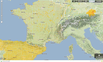
This shows the result when represented in a map (click to see it bigger). Or better use this application to browse the data for yourself (development server).

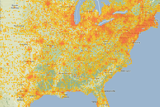
This is all the data GBIF has from different data providers about Passer domesticus (House sparrow). You can see that Spain, France and Austria seem to have some weird data. They look like if the a gridified. Specially if you compare it to the US:

The reason is that most of the data in Spain, France and Austria (also Germany but is not shown here) is derived from UTM data or another form of "area" coordinates.

And the worst is that we can not know which data is actually grid data and what is actual points, we can only see it on a map like this.

This has some repercussions:

Errors:

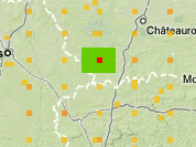
We are introducing errors to the data. The user do not know the "resolution" or quality of the data coming from GBIF. For example in France, the data in GBIF says that there is a Passer domesticus at the red point, when actually it could be in any of the greed square. Thats 25Km error from one side to the other

In Spain the error is around 10Km and in Austria is around 900m.

Visualization:

Without knowing what is a point a what is an area, it is very complicate to do any visualization that does not look strange in some areas. Experience users will understand why it might be like this, but most of the users will not. And people will keep zooming into a point thinking they can get to see the exact position of where a species was observed or collected, when actually this point is not real at all, it is just a visualization error due to the underlaying data problem.

Of course there is some works around. People are starting to share their coordinates with an error indicator. Thats good, but this is not an actual error from my point of view, it is just a different way of collecting locations, the error is in thinking that this is actually a point, when it is not, it is an area.

Fitness for analytical use:

Consider modeling predictive species distribution based on known (point) occurrence data for areas having similar environmental conditions (Environment Niche Modeling). The results of any model would be wildly inaccurate considering a 25Km deviation of input data. Some indication is necessary so that data rounded to the nearest grid is not considered valid for this use.

Possible solutions:

What possibilities we have? Well, I think the best would be to let the user share their data in the way they have it. Of course you can do that already in comments and things like that, but thats not very convenient.

So I think the best is that if people has location based on UTMs they share them like they are and also the Spatial Reference System as Well Know Text. So for example UTM10N would be:

PROJCS["NAD_1983_UTM_Zone_10N",
GEOGCS["GCS_North_American_1983",
DATUM["D_North_American_1983",SPHEROID["GRS_1980",6378137,298.257222101]],
PRIMEM["Greenwich",0],UNIT["Degree",0.0174532925199433]],
PROJECTION["Transverse_Mercator"],PARAMETER["False_Easting",500000.0],
PARAMETER["False_Northing",0.0],PARAMETER["Central_Meridian",-123.0],
PARAMETER["Scale_Factor",0.9996],PARAMETER["Latitude_of_Origin",0.0],
UNIT["Meter",1.0]]

and then they will have to share the easting and northing, like 630084m east, 4833438m north.

With this information the end user can then decide if they want to transform into lat/long if necessary, but at least they know what they are doing.

Additionally, indications that records have been rounded to a grid are required to determine their fitness for use.

I dont have experience using UTMs so I might be wrong on some of the things I have said, but at least I hope you get an idea on what the issue is and why I think is important to work on it.

Update: I should have mention that the ABCD TDWG Standard actually supports more or less what I said by providing atomic concepts for sharing UTM data. These are:

/DataSets/DataSet/Units/Unit/Gathering/SiteCoordinateSets/SiteCoordinates/CoordinatesUTM
/DataSets/DataSet/Units/Unit/Gathering/SiteCoordinateSets/SiteCoordinates/CoordinatesUTM/UTMZone
/DataSets/DataSet/Units/Unit/Gathering/SiteCoordinateSets/SiteCoordinates/CoordinatesUTM/UTMEasting
/DataSets/DataSet/Units/Unit/Gathering/SiteCoordinateSets/SiteCoordinates/CoordinatesUTM/UTMNorthing
/DataSets/DataSet/Units/Unit/Gathering/SiteCoordinateSets/SiteCoordinates/CoordinatesUTM/UTMText
/DataSets/DataSet/Units/Unit/Gathering/SiteCoordinateSets/SiteCoordinates/CoordinatesGrid
/DataSets/DataSet/Units/Unit/Gathering/SiteCoordinateSets/SiteCoordinates/CoordinatesGrid/GridCellSystem
/DataSets/DataSet/Units/Unit/Gathering/SiteCoordinateSets/SiteCoordinates/CoordinatesGrid/GridCellCode
/DataSets/DataSet/Units/Unit/Gathering/SiteCoordinateSets/SiteCoordinates/CoordinatesGrid/GridQualifier

I was part of the ABCD authors but at this time never looked much into the geospatial part of it. Now it looks to me that this is the case for a correct use of the "variable atomization" method that I did not like later on. Well, then there are cases when I like it. Of couse still work needs to be done on those concepts, and more important, people should start using them!

1234567890

Its friday the 13th and unix time will hit 1234567890 in a few hours. Well, in Continental Europe it will be saturday already, but anyone further west will be able to enjoy both at exactly Sat Feb 14 00:31:30 CET 2009

Spatial joins using PostGis

In a recent post, Tim talked about reproducing Spatial Joins using Hadoop. The reason why we started investigating on those topics is that we are cross querying the GBIF occurrence database with the Word Database on Protected Areas. The results of this work is already available for Spain, Madagascar and Tanzania. You can also check a particular protected area, like Sierra Norte in Spain. You can expect a following post about the widget developed in Flex and the visualization solution applied there.

In August we started the project only focus on Spain and Madagascar. After extracting the GBIF data that was less than 3 Million records and around 800 protected areas (polygons). With this "little" data I thought I could use some brute force and did not spend much time optimizing the processing of the data on PostGIS. In total it needed around 8 hours to analyze all data and place it in a DB schema that was enough for the service layer of the widget. These scripts are available here.

The project was very well received and soon we were asked to extend the analysis to all countries, all protected areas, and all GBIF data. That is around 90.000 protected areas and 130 million occurrences from GBIF. We knew from the beginning that the previous strategy would not scale to handle so much data and that the strategies for data representation would also not work with protected areas of the size of Spain and millions of occurrences inside. So this time we decided to go in two different ways at the same time: Using Hadoop to do the spatial join and adapt the PostGIS strategy to make it more scalable. This post is of course talking about the second strategy.

We wanted to work a little bit generic here and be able to support any kind of "polygon" analysis. That mean we would not be protected areas specific. So we have defined a Starting schema and a target schema databases. The starting schema is how we expect to get the data at the beginning and the target schema is the final processed schema that will be used to serve the data to the widget. GBIF gave us the primary data and WCMC the World Database on Protected Areas. The starting schema looks like:

The data from GBIF was given as a MySQL dump and imported into PostgreSQL using COPY statements. The WDPA on the other hand was given as a huge shapefile that we import using shp2pgsql. 

The main things we needed to process were stats on:

1. Find which GBIF occurrences are inside which polygons
2. Which providers have data for each polygons
3. Gridify the occurrences to be able to visualize them dynamically on Google Maps.
4. Construct a taxonomic tree for each polygon and grid.

So the target schema looks like this (click to expand):

The numbers in red are the number of records on each table after the data was processed.

This is the definition of main tables:

occurrence: A primary data record. The location of a species at a certain place in a certain moment.
site: Even if there are 130M occurrences they are only in around 3.5M distinct points. A site is a point on earth where an occurrence is. This just allows us to geoprocess only the distinct positions and save us lot of time.
grid10,grid5...: The grouping of the sites in cells at different scales, 10, 5,1,0.5 and 0.1 degree. After 0.1 we go dynamically grouping using PostGIS SnaptoGrid (another full post about it would be needed).

The whole processing is done using PostgreSQL and PostGIS with some new functions that we needed to create. The details about the whole process is described here . And the main steps are:

1) Adjust PostgreSQL: use 2GB of RAM. AutoVacuum Off. Use as many processors as possible.

2) Get the sites: No more than a grouping of the occurrences by coordinates.

3) Spatially join the sites with the polygon table: This is where it gets interesting. The fastest way we found was using the distance function and run it threaded in parallel in different parts of the site. This is a  computer intensive task so I used the 8 cores in my computer. The task takes around 4 hours. But depend s a lot on the complexity of the polygons and how good you are at distributing the load among different processors. We used a PHP script and a shell script to run several queries at the same time.

4) Delete sites that are not inside polygons and later delete the occurrences that are not in sites.

5) Create the grids: we are using our own grid system based on work previously done by Tim Robertson. The way we group the sites on the occurrences is by spatially joining the sites against tables with all the grid cells pre-created. To generate the grids Tim developed a little Java tool that create PostGIS insert statements. It is the GridBuilder class .  But if someone needs them we can provide them directly as zip SQL files.

6) Generate stats: Calculate the number of occurrences, species, specimens, observations, other basis of records, plants, animals and other kingdoms. Those stats are available per polygon, per grid, per site, per provider, per taxon, etc... Lot of queries but that run very fast.

7) Generate taxonomy for each polygon: this can be a complicate process. The idea is to generate classifications per polygon based on the occurrences that are inside these polygons. We have created a PostgreSQL function that scan the occurrence table per polygon and generate the  classification. The source code of this function is here .

And this is more or less everything. Of course lot of details are skipped here, like when to vacuum, generate indexes, etc. But you can find most of these details on the description page of this strategy .

You can find in any case all the source code for all those things on the Google Code GBIF-WDPA project. There you will find the source code of the Java SOA application, the Flex source code of the widget, the processing scripts and comments, well, everything created during this project.
we are working on a single script that will run the full process in one shot and it will be available there when ready.

Summary:
Well, after this long post my main recomendations if you need to use PostGIS to do something similar would be:
-Adjust postgreSQL settings regarding memory.
-Consider threading long operations that require a huge table scan.
-"Create table as" is much faster than updating.
-Amazon Web Services can be very slow due to I/O performance issues.
-Buy a Wii to play while you wait for results :)

Leave us a comment if you have any question or suggestions regarding this processing strategy.

And finally happy christmas everybody!

Reproducing Spatial Joins using Hadoop and EC2

Finally I got some time to continue researching the use of Hadoop for the processing of the GBIF dataset with respect to the protected areas of the world.

The problem
There is a growing number of point data, and an increasing need to perform cross referencing of the GBIF data with external sources, in this case the protected areas of the world.

The last 3 years of working on reasonably large databases (>100G) has told me that this join was not going to be an easy one, despite the obvious partitioning strategy that can be invoked here (spatial partitioning).
Therefore Javi and I set about this task by

1. Using PostGIS and the traditional approach of joining 2 tables of 150M point records with 120,000 polygon records - finding will be posted shortly
   
2. Using Hadoop and the Amazon EC2 to process the join

Using Hadoop
This is ongoing but I thought I'd post the findings so far.

Strategy 1: 

Partition by cell
Start by splitting the 150M records from one file into a file per 1 degree cell.
Loop over each polygon:

• Determine 1 degree cells covered polygon
  
• Use the input files as a merge input to hadoop and pass in the Polygon for the Map to do the contains()
  

Result  

Hadoop will not handle so many file splits no matter what configuration I try so far. Mailing list responses suggest this is not the ideal use of Hadoop and it prefers single large files, rather than many smaller ones.

Amendment

Using 10 degree cells, it does work but takes a LONG time... so long I killed it. This was expected since it is really the equivalent of only a DB join with an index on an INTEGER teg_deg column.

Strategy 2: 

1-Degree in-memory index of polygons
So this approach goes through the join the opposite way. The polygons are loaded into memory and a

HashMap<Integer, Collection<Polygon>>

for each Map operation to use.  

The logic is effectively give me polygons intersecting the 1 degree square for this point, and then test them properly. This worked ok, but requires a LOT of memory for the polygons to be held.

Result

About 6 hours to process 60,000 polygons.

Strategy 3: 

RTree index of polygons
Very similar to strategy 2, this approach indexes all the polygons by RTree. Thus for each point, the index provides only candidate polygons whose bounding box contains the point, and the number of candidate polygons to test is far smaller than that of strategy 2.

Result

45 minutes for a 130M x 30,000 cross reference but requires the larger EC2 instance sizes. The RTree index means it will need processed in batches.
Hadoop requires tuning, just like a database does for large joins. Here is the final tuning for strategy 3:

• mapred.child.java.opts=-Xmx1G // for the R-Tree index
• mapred.output.compress=false // for easy reading of output
• mapred.tasktracker.map.tasks.maximum=4 // we have 7G per node, so 4G for 4 Map tasks is ok
• mapred.job.reuse.jvm.num.tasks=-1 // Reuse the Map as it has the index built (takes 90 seconds for startup)
• dfs.block.size=134217728 // use larger blocks - in retropsect this was a probable mistake and will be removed for next test

More to follow...

Thanks to the Hadoop-core Users mailing list for their insights, and Andrea of OpenGEO for pointing me at the JTS RTree implementation

Do you know any species distribution project?

I am trying to create a general view on how species distributions are handle in different projects world wide. I am specially interested in project where they have maps and are published on Internet. So I would like to ask you for links to projects related to Species Distributions.

I am also interested in different ways people handle occurrence status or absence. 

And finally I also would like links to any mapping application that you have seen related to Species distributions. And if possible comment what you liked.

Please post your links as comments to this post or send them to me (jatorre@gmail.com). I will post in the future the results from this little research.

Thanks!

Flickr creating polygons out of points, what about species distributions?

This weekend I have found a very interesting post from the Flickr programmers called The shape of Alpha. What this people are basically doing is generating shapefiles from the geotagged pictures in Flickr. When a user geotag a picture, provide lat/long, they reverse-geocode it to find the neighborhood, the town, the country etc where this coordinates are.  They store this information in the database (as  Where On Earth(WOE) IDs) and this allow for much better performance when later people search for pictures in "Madrid".

But this post talks about a different idea, and it is awesome. Now that they have all this geotagged pictures and they know they are in a particular neighborhood or country (WOEID) they are creating shapefiles from these areas based on the coordinates of the different pictures! Maybe is easier to explain it with a picture:

The one in the left is a London polygon and the right for United States. They were created by aggregating all the coordinates of the different pictures found in London and in the US.

Again. They take all the coordinates, POINTs, in the DB for a certain WOEID and with them they generate a polygon. If they have enough data it looks more or less ok. They have a good discussion about the quality of the polygons and the threshold set to generate them. I like very much the introduction they make to  Alpha shapes and the links they provide.

Additionally they also provide the source code of the tool they use to process the data. It is called Clustr.

Now, lets apply this concept to Biodiversity, if you haven't already figure it out. Think of their geotagged pictures as PRIMARY DATA, the WOE as SCIENTIFIC NAMES and the polygons you get out of them as DERIVED SPECIES DISTRIBUTION polygons.

I have been investigating this for a long time already, specially trough the Biodiversity Atlas project that is now stopped, but hopefully will start soon. We can take their source code and apply it to GBIF data and generate "derived, unchecked and uncompleted" species distributions based on GBIF data on a massive way! And the same they try in Flickr, the more primary data we get into the system the better the distributions will start looking like.

But there is another idea... why dont ask Flickr to not only process their polygons based on WOE Ids but also on tags? So if we tag pictures in Flickr with scientific names, or better GUIDs, they can then try to generate by themselves the distributions.

I particularly dont see Flickr as the best place to handle species distributions discussions, and will, hopefully, try to convince at least one big biodiversity project to let me try this way. Most of you can probably imagine the incredible API we can create once we have a lot of species distributions accessible in such a system. I will write another post about it soon, but think of:

• Which species could live in my garden?
• Which species habitats this new road will cross? 
• Where should I create a new Protected Area to preserve as much biodiversity as possible?
• What species could I find in the track I will hike this weekend?

So maybe instead of so much niche modeling projects we should start thinking on how to manage the vast amount of primary data (and other sources) we have already  and how to curate it and complete it. I dream of a scientific community joined together to create a complete information system to know where species are. Imagine like a Wikipedia but for Species Distributions.