WMS Tiling Clients

For projects relying on open source software and using WMS services for their map applications perhaps the most obvious choice for a client application is to write something using the OpenLayers API. This is a very extensive javascript API and is used to demonstrate the open source OGC compliant servers MapServer and GeoServer. Its straight forward to construct a map and then to overlay multiple layers using WMS services.

The screenshot above shows a layer of 0.1 degree cell densities representing data from Australian National Herbarium rendered using GeoServer layered on top of the Google satellite base layer, all pulled together using OpenLayers.

Running this locally the map was rendered by OpenLayers rather quickly. Running this on an externally hosted server I began to notice curious loading of tiles by OpenLayers. So I did a stripped down comparison of the same functionality using the Google maps API. Rendering the cell density tiles from a WMS service in Google maps was done using a javascript function written by John Deck - available here.

The performance improvement with Google maps was immediately obvious. Using the Firefox YSlow plugin we see:

OpenLayers	Google Maps API

So the main thing of interest here is the number of tiles loaded by OpenLayers compared to Google maps (91 vs 50 - although oddly the total size of the images loaded is roughly equivalent, and the tile size for both seems to be 256x256 pixels). Increasing the size of the tile for OpenLayers does reduce the number of tiles requested (I tested with 512x512 and 1024x1024) but this has little effect on performance in openlayers.

So the performance difference between Google Maps and OpenLayers could be accounted for by any combination of the following:

• Incorrect use of the API (test for OpenLayers is here) and we are missing configuration to reduce tile loading in openlayers
  
• The tile loading algorithm for Google maps is more efficient in only loading the required tiles for selected view areas
• Openlayers is preloading more images to speed up panning. This would be good, but OpenLayers doesnt seem to prioritise the loading of currently viewed tiles.
  

The source for the test for OpenLayers is here, and for Google maps here.

The Taxonomy browser visualization #1 - Tree Lists

Hi, my name is Sergio Alvarez Leiva and this is my first pos at biodivertido, Finally. I'm part of Vizzuality and work as Interaction Designer for GBIF among others. I will mainly be posting about Interaction Design, UX and Design in general, althought I'll try to post about Front.end developing a little. I hope you find it interesting.

Since I began designing for Biodiversity data, I've encountered lot of interesting challenges related to the size of the datasets .

Maybe, one of the hardest challenges is designing a taxonomy browser visualization. The taxonomy browser can represent up to 1.7M names, with nodes with more than 200 childs. That makes it complicate in terms of interaction design and performance.

I will write in a series of post my impressions on different techniques we have been experimenting:

In this first post I'm going to talk about tree list visualizations, but before I get into details, I'd like to talk a little about generic concepts that might be applied to all the visualizations. There is a lot of bibliography about trees out there, but let me introduce here my own "easy" concepts.

When browsing a tree you need to know where you are and what is around you, thats parent and brothers and in general this is called Contextualization. Then you need to be able to find the childs, thats Discovering. All this needs to be easy to do, Usability and UX, and finally must be easy to integrate with the application, Easy integration.

On those terms, the tree list visualization presents some advantages and disadvantages.

- Contextualization: Maybe the list visualization is the most standard way to solve this problem. The tree lists lets the user discover the whole tree by clicking in the different nodes. But the problem is the vertical size that the tree gets when the user deployes a node (This is an integration problem too). When the user will have deployed more than 3 levels, he will have to use the vertical scroll, and probably, this action will make the contextual information (parent nodes and "brothers") out of the visible screen area.

This problem could be solved implementing some variations in the Tree list; We could hide all the nodes not related to the selected child and get more space for view only the important nodes.

-Poor UX : "Discovering biodiversity". We have to involve the users in our play and invite they to discover more and more. I think the Tree Lists are a little boring...we need more action!

- Usability: This visualization is pretty used and the users will understand how it works quickly. On the other hand, I think that in a Tree list is not so easy to find the desired node - the users would have to deploy a lot of nodes, and scroll a lot too, before find their objective. Maybe would be positive for this point to implement a search box. It might depend of the data size.

Conclusion; We've a standard visualization that lets us to implement a Taxonomic browser in a lot of different situations. I think this is not the best solution that we could implement, but its true that we could use this always. 

 

SpatialKey and biodiversity primary data analysis

Some days ago the good people from Universal Mind open the beta program for their new product called SpatialKey. For those who are not in the Flex community, Universal Mind is a very recognized company developing Rich Internet Applications. So it was a great pleasure when I saw months ago that they were working on a new geospatial product for data analysis.

I was lucky to get an invitation to the beta program and be able to take a look. They are promising some great things, but for the moment the beta is limited in certain ways I will describe later. The best to get an overview of it is to watch some of their ubercool videos (maybe too much for my taste).

I wanted to give it a try as soon as possible, and coincidentally I just finished working on the new WDPA-GBIF widget. The widget allows you to visualize biodiversity primary data, from GBIF, for all protected areas in the world. Check out for example the protected areas in Australia. Then select for example an area like the Great Barrier Reef. You will be able to download the data in multiple formats.

With this I downloaded the data for the Canadian Rocky Mountains and imported it in SpatialKey. The import now is limited to 10.000 records and 25 columns, so I had to delete multiple columns and records. I think SpatialKey should allow the discard of the data visually when it is already uploaded.

With SpatialKey you manage separately your datasets and the reports you create based on them. The reports right now are not exportable to the outside. I mean, you can not print or distribute as a widget the report you have created. I know they are working on it, but for the time being I only have 2 possibilities to show you how it looks like: share my report with everybody that gives me his email, or just do a little screencast for everybody to watch here. For the first one if someone is really interested to get into the system to take a look, send me an email. the screencast is following:

So here goes the things that I like a lot:

• The heatmaps are just gorgeous. I would love to know how they do it.
• The timeline filter is great. Has some usability issues but is great.
• The way grids are displayed for summaries. The hover effect is very good and the tooltip very clear.
• The filter "pods" are nice, but I wonder what would happen when you have thousands of hundreds records to search or select on. I suppose that when there is lot of data only the search would be enabled and not the selection.
• Great look and feel.

Other comments following:

• Is it necessary to refresh on every map movement? I understand it is on the zoom and if you have the filter by visible area disabled.
• Not having the possibility right now to share the reports as widgets to embed on the blog.
• It would be nice to also let the user provide a polygon or geometry to define the boundaries of the analysis. In this case for example would help a lot to visualize the borders of the protected area.

And finally, the things I really wonder how they work internally:

• The heatmaps!
• The data structures they use for dynamically regrouping the data on the client.
• If it is true that they can handle millions of records, how does the server infrastructure looks like. I know it is Java, but what about the data store, how can they handle the creation of dynamic indexes or how do they do it? Would it work with GBIF data?

My general impression of the tool is great. It looks awesome and works really well. It looks very similar to some of the ideas we have for developing analytical tools for biodiversity data with GBIF. Tim give your impressions please!

I would love to see more and more such analytical tools for biodiversity. How they call them? Something like Bussiness Intelligence, I think we need some of this in our community. For the time being I will try to get into talks with Universal Mind on the applicability of SpatialKey for huge biodiversity primary data like GBIF.

How many zoom levels are enough?

While processing the GBIF data index for all species to display the maps shown in the last post I though it worth showing the number of "occurrences per species per cell" at the various zoom levels.
We make use of the tiling mechanism employed by many mapping clients, who request 256x256 pixel tiles and then we process the data to be several zoom levels ahead of the one displayed.  It is really quite simple, and best described with a couple of examples. 

Processing to 4 zoom levels ahead looks like:

Processing to 6 zoom levels ahead looks like:

When processing to 6 zoom levels, the following shows where it becomes unnecessary to process anymore (around zoom level 11):

Grid data shared as point data. Errors and visualization problems

In todays world the easiest way to share location is using Decimal latitude and longitudes, and preferably on WGS84. With such coordinates you can make use of lot of existing data transfer standards, mapping APIs, or analysis tools. This is good because it helps a lot on interoperability and let developers and scientist easily mix data and use it together.

But, most of biodiversity primary data, the location of a species at a certain place in a certain moment, was taken before GPS and even after lot of different coordinate systems were used. For example UTM. In those coordinates systems people do not indicate an exact position, like you do with lat/lon, but an area or zone. That is ok for most uses, you dont need to know the exact position of where a specimen was collected, and sometimes it is even much easier to use those zones, or cells or area, to collect and aggregate data.

The problem comes when you start sharing your data in public networks like GBIF. Most of data providers in the GBIF network, if not all, provide their data using lat/long. This is even the recommended method to easier process and aggregate the data. Therefore what most providers are doing is transforming those areas into points by taking the centre of the area.

If you put this transformed coordinates with other real lat/long coordinates, like GBIF does, then you end up not knowing what was originally a cell or an area and what was really a point.

This shows the result when represented in a map (click to see it bigger). Or better use this application to browse the data for yourself (development server).

This is all the data GBIF has from different data providers about Passer domesticus (House sparrow). You can see that Spain, France and Austria seem to have some weird data. They look like if the a gridified. Specially if you compare it to the US:

The reason is that most of the data in Spain, France and Austria (also Germany but is not shown here) is derived from UTM data or another form of "area" coordinates.

And the worst is that we can not know which data is actually grid data and what is actual points, we can only see it on a map like this.

This has some repercussions:

Errors:

We are introducing errors to the data. The user do not know the "resolution" or quality of the data coming from GBIF. For example in France, the data in GBIF says that there is a Passer domesticus at the red point, when actually it could be in any of the greed square. Thats 25Km error from one side to the other

In Spain the error is around 10Km and in Austria is around 900m.

Visualization:

Without knowing what is a point a what is an area, it is very complicate to do any visualization that does not look strange in some areas. Experience users will understand why it might be like this, but most of the users will not. And people will keep zooming into a point thinking they can get to see the exact position of where a species was observed or collected, when actually this point is not real at all, it is just a visualization error due to the underlaying data problem.

Of course there is some works around. People are starting to share their coordinates with an error indicator. Thats good, but this is not an actual error from my point of view, it is just a different way of collecting locations, the error is in thinking that this is actually a point, when it is not, it is an area.

Fitness for analytical use:

Consider modeling predictive species distribution based on known (point) occurrence data for areas having similar environmental conditions (Environment Niche Modeling). The results of any model would be wildly inaccurate considering a 25Km deviation of input data. Some indication is necessary so that data rounded to the nearest grid is not considered valid for this use.

Possible solutions:

What possibilities we have? Well, I think the best would be to let the user share their data in the way they have it. Of course you can do that already in comments and things like that, but thats not very convenient.

So I think the best is that if people has location based on UTMs they share them like they are and also the Spatial Reference System as Well Know Text. So for example UTM10N would be:

PROJCS["NAD_1983_UTM_Zone_10N",
GEOGCS["GCS_North_American_1983",
DATUM["D_North_American_1983",SPHEROID["GRS_1980",6378137,298.257222101]],
PRIMEM["Greenwich",0],UNIT["Degree",0.0174532925199433]],
PROJECTION["Transverse_Mercator"],PARAMETER["False_Easting",500000.0],
PARAMETER["False_Northing",0.0],PARAMETER["Central_Meridian",-123.0],
PARAMETER["Scale_Factor",0.9996],PARAMETER["Latitude_of_Origin",0.0],
UNIT["Meter",1.0]]

and then they will have to share the easting and northing, like 630084m east, 4833438m north.

With this information the end user can then decide if they want to transform into lat/long if necessary, but at least they know what they are doing.

Additionally, indications that records have been rounded to a grid are required to determine their fitness for use.

I dont have experience using UTMs so I might be wrong on some of the things I have said, but at least I hope you get an idea on what the issue is and why I think is important to work on it.

Update: I should have mention that the ABCD TDWG Standard actually supports more or less what I said by providing atomic concepts for sharing UTM data. These are:

/DataSets/DataSet/Units/Unit/Gathering/SiteCoordinateSets/SiteCoordinates/CoordinatesUTM
/DataSets/DataSet/Units/Unit/Gathering/SiteCoordinateSets/SiteCoordinates/CoordinatesUTM/UTMZone
/DataSets/DataSet/Units/Unit/Gathering/SiteCoordinateSets/SiteCoordinates/CoordinatesUTM/UTMEasting
/DataSets/DataSet/Units/Unit/Gathering/SiteCoordinateSets/SiteCoordinates/CoordinatesUTM/UTMNorthing
/DataSets/DataSet/Units/Unit/Gathering/SiteCoordinateSets/SiteCoordinates/CoordinatesUTM/UTMText
/DataSets/DataSet/Units/Unit/Gathering/SiteCoordinateSets/SiteCoordinates/CoordinatesGrid
/DataSets/DataSet/Units/Unit/Gathering/SiteCoordinateSets/SiteCoordinates/CoordinatesGrid/GridCellSystem
/DataSets/DataSet/Units/Unit/Gathering/SiteCoordinateSets/SiteCoordinates/CoordinatesGrid/GridCellCode
/DataSets/DataSet/Units/Unit/Gathering/SiteCoordinateSets/SiteCoordinates/CoordinatesGrid/GridQualifier

I was part of the ABCD authors but at this time never looked much into the geospatial part of it. Now it looks to me that this is the case for a correct use of the "variable atomization" method that I did not like later on. Well, then there are cases when I like it. Of couse still work needs to be done on those concepts, and more important, people should start using them!

1234567890

Its friday the 13th and unix time will hit 1234567890 in a few hours. Well, in Continental Europe it will be saturday already, but anyone further west will be able to enjoy both at exactly Sat Feb 14 00:31:30 CET 2009

Spatial joins using PostGis

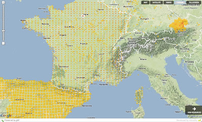
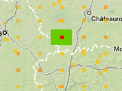
In a recent post, Tim talked about reproducing Spatial Joins using Hadoop. The reason why we started investigating on those topics is that we are cross querying the GBIF occurrence database with the Word Database on Protected Areas. The results of this work is already available for Spain, Madagascar and Tanzania. You can also check a particular protected area, like Sierra Norte in Spain. You can expect a following post about the widget developed in Flex and the visualization solution applied there.

In August we started the project only focus on Spain and Madagascar. After extracting the GBIF data that was less than 3 Million records and around 800 protected areas (polygons). With this "little" data I thought I could use some brute force and did not spend much time optimizing the processing of the data on PostGIS. In total it needed around 8 hours to analyze all data and place it in a DB schema that was enough for the service layer of the widget. These scripts are available here.

The project was very well received and soon we were asked to extend the analysis to all countries, all protected areas, and all GBIF data. That is around 90.000 protected areas and 130 million occurrences from GBIF. We knew from the beginning that the previous strategy would not scale to handle so much data and that the strategies for data representation would also not work with protected areas of the size of Spain and millions of occurrences inside. So this time we decided to go in two different ways at the same time: Using Hadoop to do the spatial join and adapt the PostGIS strategy to make it more scalable. This post is of course talking about the second strategy.

We wanted to work a little bit generic here and be able to support any kind of "polygon" analysis. That mean we would not be protected areas specific. So we have defined a Starting schema and a target schema databases. The starting schema is how we expect to get the data at the beginning and the target schema is the final processed schema that will be used to serve the data to the widget. GBIF gave us the primary data and WCMC the World Database on Protected Areas. The starting schema looks like:

The data from GBIF was given as a MySQL dump and imported into PostgreSQL using COPY statements. The WDPA on the other hand was given as a huge shapefile that we import using shp2pgsql. 

The main things we needed to process were stats on:

1. Find which GBIF occurrences are inside which polygons
2. Which providers have data for each polygons
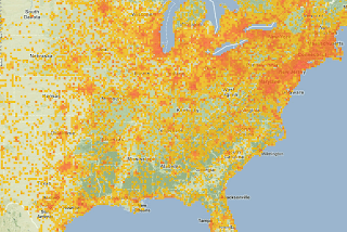
3. Gridify the occurrences to be able to visualize them dynamically on Google Maps.
4. Construct a taxonomic tree for each polygon and grid.

So the target schema looks like this (click to expand):

The numbers in red are the number of records on each table after the data was processed.

This is the definition of main tables:

occurrence: A primary data record. The location of a species at a certain place in a certain moment.
site: Even if there are 130M occurrences they are only in around 3.5M distinct points. A site is a point on earth where an occurrence is. This just allows us to geoprocess only the distinct positions and save us lot of time.
grid10,grid5...: The grouping of the sites in cells at different scales, 10, 5,1,0.5 and 0.1 degree. After 0.1 we go dynamically grouping using PostGIS SnaptoGrid (another full post about it would be needed).

The whole processing is done using PostgreSQL and PostGIS with some new functions that we needed to create. The details about the whole process is described here . And the main steps are:

1) Adjust PostgreSQL: use 2GB of RAM. AutoVacuum Off. Use as many processors as possible.

2) Get the sites: No more than a grouping of the occurrences by coordinates.

3) Spatially join the sites with the polygon table: This is where it gets interesting. The fastest way we found was using the distance function and run it threaded in parallel in different parts of the site. This is a  computer intensive task so I used the 8 cores in my computer. The task takes around 4 hours. But depend s a lot on the complexity of the polygons and how good you are at distributing the load among different processors. We used a PHP script and a shell script to run several queries at the same time.

4) Delete sites that are not inside polygons and later delete the occurrences that are not in sites.

5) Create the grids: we are using our own grid system based on work previously done by Tim Robertson. The way we group the sites on the occurrences is by spatially joining the sites against tables with all the grid cells pre-created. To generate the grids Tim developed a little Java tool that create PostGIS insert statements. It is the GridBuilder class .  But if someone needs them we can provide them directly as zip SQL files.

6) Generate stats: Calculate the number of occurrences, species, specimens, observations, other basis of records, plants, animals and other kingdoms. Those stats are available per polygon, per grid, per site, per provider, per taxon, etc... Lot of queries but that run very fast.

7) Generate taxonomy for each polygon: this can be a complicate process. The idea is to generate classifications per polygon based on the occurrences that are inside these polygons. We have created a PostgreSQL function that scan the occurrence table per polygon and generate the  classification. The source code of this function is here .

And this is more or less everything. Of course lot of details are skipped here, like when to vacuum, generate indexes, etc. But you can find most of these details on the description page of this strategy .

You can find in any case all the source code for all those things on the Google Code GBIF-WDPA project. There you will find the source code of the Java SOA application, the Flex source code of the widget, the processing scripts and comments, well, everything created during this project.
we are working on a single script that will run the full process in one shot and it will be available there when ready.

Summary:
Well, after this long post my main recomendations if you need to use PostGIS to do something similar would be:
-Adjust postgreSQL settings regarding memory.
-Consider threading long operations that require a huge table scan.
-"Create table as" is much faster than updating.
-Amazon Web Services can be very slow due to I/O performance issues.
-Buy a Wii to play while you wait for results :)

Leave us a comment if you have any question or suggestions regarding this processing strategy.

And finally happy christmas everybody!